Paper Summary: Simple Model of Spiking Neurons (Izhikevich 2003)

In this post I am summarising “Simple Model of Spiking Neurons” by Izhikevich (2003), you can find more information about this work here.

Assumed Knowledge

I will try to make the post accessible to a general audience, but in the interest of brevity I wont explain every concept from scratch. For this post it may be helpful to know about:

• Basic artificial neural networks such as the multi-layer perceptron

Background and motivation

The work proposes a biological/spiking neuron model. Such models emulate the biochemical process which underlie neural activity. Of particular interest is how these processes combined in a network of neurons propagate and process information through bursts of activity in cell voltage called spikes. The goal is to develop our understanding of the brain through large scale simulation of spiking neural networks, and to use these networks in artificial intelligence systems (example I read recently).

The key contribution over previous models such as the Hodgkin-Huxley model is a significant increase in computational efficiency, without sacrificing the desired biological accuracy (w.r.t. observed spiking patterns). To quantify, it is possible to run 10s of Hodgkin-Huxley neurons in real time, Izhikevich showed his model could easily simulate a 10,000 neuron network (1,000,000 connection) using an old (in 2003) 1 GHz PC.

The work in detail

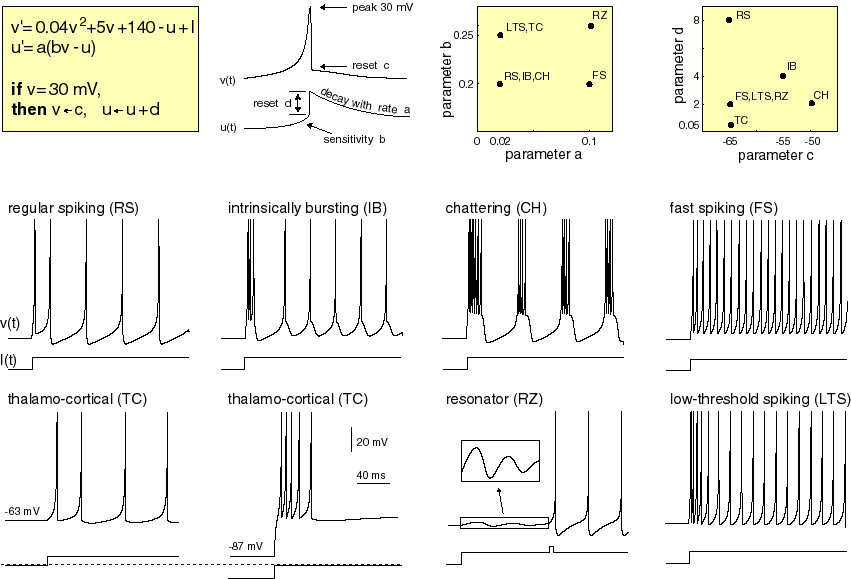
The model consists of two differential equations (v', u') controlling the transformation of the membrane potential (v) and a recovery variable (u) which acts to inhibit spike generation for some time after a spike.

Given an input stimulus current (I) the voltage of the neuron increases until a critical spiking threshold (30mV), at this point the voltage is instantly reset and the inhibitory recovery variable is increased (thus delaying the next spike).

By using different combinations of the four parameters (a, b, c, d), diverse spiking behaviour corresponding to naturally observed spike patterns can be generated. These parameters perform the following function:

• a: Scales the transformation of the recovery variable, larger values means the neuron can fire more often. e.g. regular spiking vs. fast spiking.
• b: Changes the extent to which the current membrane potential (v) affects the transformation of the recovery variable.
• c: The value which the membrane potential (v) is reset to after the threshold is reached.
• d: The offset applied to the recovery variable (u) after the threshold is reached, to inhibit subsequent spiking.

Image source here.

The work demonstrates how a network of such neurons may be used to simulate observed neural activity. The network is split into excitatory and inhibitory neurons (in this case a 4:1 ratio). The generation of a spike in an excitatory neuron increases the input current (I) of connected neuron. Conversely, inhibitory neurons decrease the input current. The strength of this increase/decrease is based on an assigned synaptic weight which is assigned randomly. Additionally, inhibitory connections are twice as strong as excitatory ones in this case.

The excitatory and inhibitory neurons also use different parameter settings and therefore exhibit different firing patterns. This roughly corresponds to the regular spiking and fast spiking patterns respectively. However behavioural variance is introduced by randomising the parameters around these patterns. The below code from my implementation demonstrates the initialisation of the network:

    ## Create network
    neurons = [] 
    S = [] # synaptic connection strengths
    for i, r in enumerate(rx):

        # create neuron as per ranges defined in Izhikevich
        if i < Ne: # is excitatory
            neurons.append(INeuron(0.02, 0.2, -65.0 + (15.0 * (r**2)), 8.0 - (6.0 * (r**2))))
        else:
            neurons.append(INeuron(0.02 + (0.08*r), 0.25 - (0.05*r), -65.0, 2.0))

        # create connections
        ws = [ random.random() for _ in range(total)]
        for j in range(total):
            if i < Ne: # is excitatory
                ws[j] = ws[j] * 0.5 # weaker
            else:
                ws[j] = ws[j] * -1 # inhibit
        S.append(ws)

I ran this network for 500ms which gave the below firing pattern. With considerable variance there is an overall concentration of activity every ~100ms. The work suggests that by modifying the network configuration, the ratio of excitatory/inhibitory neurons, and the synaptic weights interesting patterns corresponding to real neural activity can be observed.

You can find my Python implementation of the Izhikevich model on GitHub here, and the original MATLAB code on the author’s website

Extensions and applications

The key contribution of this work is vastly increasing the computational efficiency of biologically plausible spiking neural networks. For the study of natural systems this means simulating more complex regions of the brain in reasonable timeframes. For AI this means the possibility of applying spiking neural networks in intelligent systems.

The trick with any artificial neural network is determining the network configuration (neurons and connections) and parameter assignment (weights, etc.) which will lead to some useful overall behaviour. With current abstract models the popular technique for learning connection weights uses some form of error backpropagation. Such techniques cannot be directly applied in spiking neural networks where information is propagated through state dependent spike generation rather than the relatively simple numerical output state of the abstract model.

Izhikevich’s work did not discuss techniques for such learning, but others have suggested methods to achieve this such as spike-timing dependent plasticity. The possible advantage of this type of network over popular abstract models, and techniques for determining network configuration and connection parameters are topic of my own future investigation. This investigation would not be possible without a computationally tractable model as outlined by Izhikevich.